FIR filter design experiment using the simplex method

Philippe Strauss

2010-09-01 00:00

A starter about symetrical (linear phase) finite impulse response digital filter design using the simplex method. Much slower than Parks/McClellan/Remez exchange, but packaged in GLPK. 75 lines of OCaml code to design an FIR filter, what less could you ask for ?

The paper to have in hands is the "Meteor" one by Steiglitz. In short, from a vector dot matrix multiplication, we get the frequency response. The matrix beeing a cosine table, the vector beeing the filter coefficients.

The simplex method beeing a relatively simple optimization procedure for linear problems.

Building

You need ocaml-glpk, ocaml-gnuplot. Using findlib, I build it with:

ocamlfind opt -o simplex_fir -package glpk,gnuplot -linkpkg
simplex_fir0.ml -ccopt \"-L/opt/local/lib\"

(* A first experiment with the simplex method for FIR filter design
   Philippe Strauss, philou at philou.ch, 2010 *)
open Glpk
module P = Gnuplot.Array

type trigf = Cosine | Sine

let foi = float_of_int

let pi = 4. *. (atan 1.)

let trig fct f harm =
    let om = 2. *. pi *. f *. (foi harm) in
    match fct with
    | Cosine -> cos om
    | Sine -> sin om

(* _T for transposed, about the vector *)
let mul_mat_vect_T a x =
    let lena_l = Array.length a in
    let lena_c = Array.length (a.(0)) in
    let lenx = Array.length x in
    assert (lena_c = lenx) ;
    let mul = Array.make lena_l 0. in
    for i = 0 to lena_l - 1 do
        let a_i = a.(i) in (* hoisting *)
        let accum = ref 0. in
        for j = 0 to lenx - 1 do
            accum := !accum +. x.(j) *. a_i.(j)
        done ;
        mul.(i) <- !accum ;
    done ;
    mul

let init_trig_table fct nf ncol =
    let tbl = Array.make_matrix nf ncol 0. in
    let fstep = 0.5 /. (foi nf) in
    for i = 0 to nf - 1 do
        for j = 0 to ncol - 1 do
            tbl.(i).(j) <- trig fct (fstep *. (foi i)) j
        done ;
    done ;
    tbl

let () =
    let ncoeffs = 151 in
    let ncoeffs2 = (ncoeffs - 1) / 2 in
    let nf = 1000 in
    let a = init_trig_table Cosine nf ncoeffs2 in
    let fstep = 0.5 /. (foi nf) in
    let target_mag_response f =
        if f < 0.15 then (0.99, 1.01)
        else if f < 0.18 then (0.0, 1.01)
        else (-0.00001, 0.00001)
    in
    let pbounds0 = Array.make nf (-.infinity, infinity) in
    let pbounds = Array.mapi (fun i x -> target_mag_response (fstep *. (foi i))) pbounds0 in
    let zcoeffs = Array.make ncoeffs2 1. in
    let xbounds = Array.make ncoeffs2 (-.1., 1.) in
    let lp = make_problem Maximize zcoeffs a pbounds xbounds in
    scale_problem lp ;
    use_presolver lp true ;
    simplex lp ;
    let coeffs = get_col_primals lp in
    for j = 0 to Array.length coeffs - 1 do
        Printf.printf "%4d = %.5f\n" j coeffs.(j) ;
    done ;
    let mag = mul_mat_vect_T a coeffs in
    let mag_db = Array.map (fun x -> 10. *. (if x = 0.0 then (-20.) else log10 (x ** 2.))) mag in
    let freq = Array.init nf (fun i -> foi i *. 0.5 /. foi nf) in
    let g = P.init ~xsize:800. ~ysize:400. Gnuplot.X in
    P.title g "Amplitude response" ;
    P.xlabel g "Freq" ;
    P.env g ~xlog:true 0.001 (0.5) (-120.) 10.;
    P.ylabel g "Amplitude [dB]" ;
    P.pen g 1 ;
    P.xy g freq mag_db ;
    P.close g

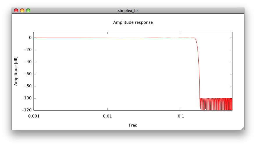
Here's a screenshot of the gnuplot invocation, showing the frequency response when no truncation of coefficients occurs (float32 is much enough accuracy here):

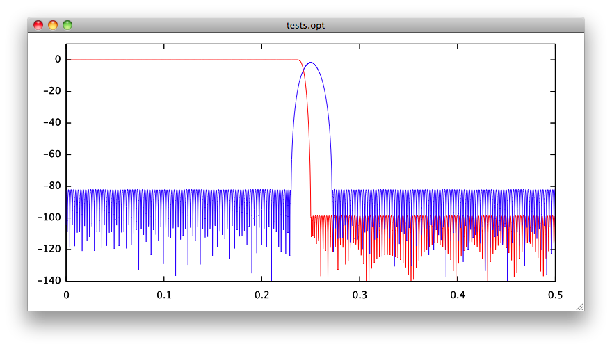
And for comparison, two FIR filters designed using the classical Remez exchange algorithm, one of 371 taps in red, the blue one beeing of 401 taps.

Philippe Strauss website

Building

Comments